What Is a Feedforward Neural Network?

A feedforward neural network is the foundation of all applied deep learning — and the right starting point for most business ML projects. Understanding how data flows through these networks, how they learn, and when to use them gives you a clear framework for evaluating any AI implementation.

What Is a Feedforward Neural Network?

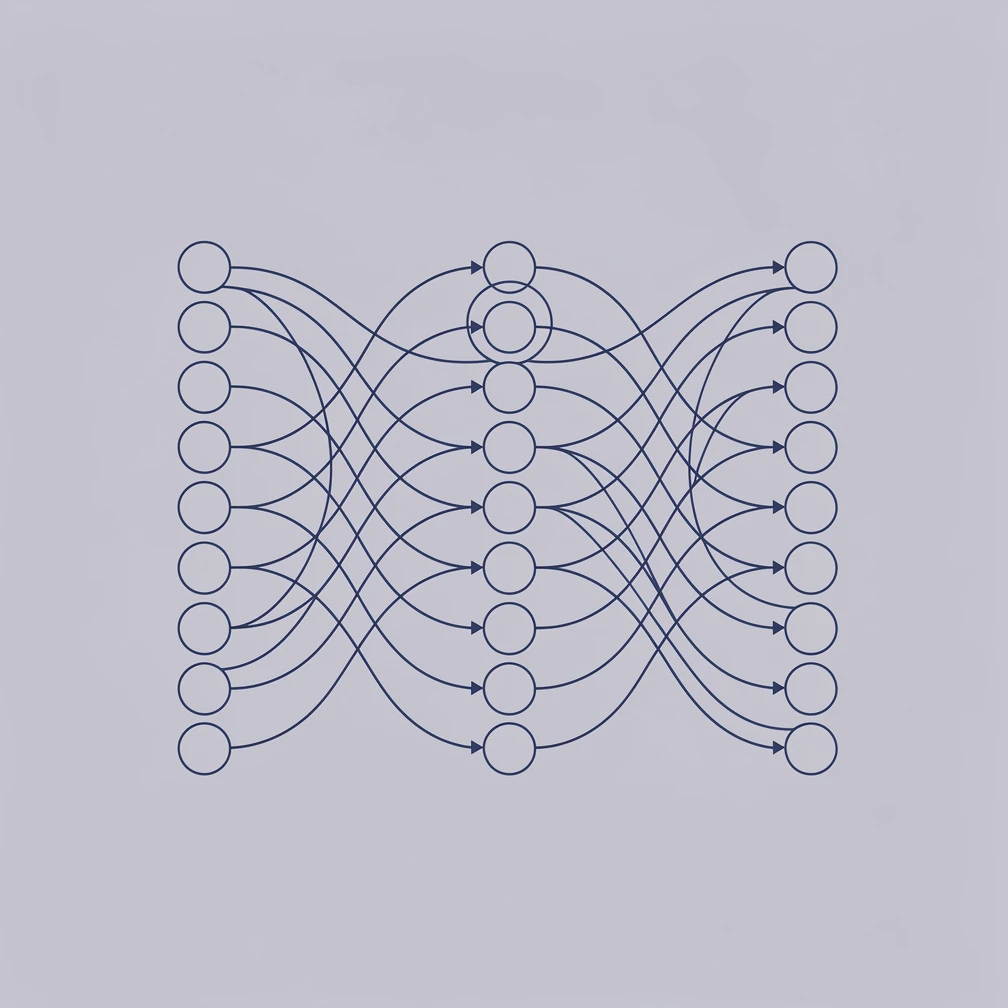
A feedforward neural network processes data in a single direction: from input nodes through one or more hidden layers to an output prediction, with no loops or cycles. Each layer applies a mathematical transformation — weighted sums plus activation functions — before passing results forward. The multilayer perceptron (MLP) is the standard business-ready variant, capable of classification, regression, and ranking tasks on structured data.

The “feedforward” name describes the information flow. Unlike recurrent neural networks, which loop outputs back as inputs to retain sequence memory, feedforward networks treat every input independently. This makes them fast, parallelizable, and well-suited to tabular data — the kind of structured rows and columns that businesses produce in CRM systems, transaction databases, and sensor logs.

The Three Layers of Every Feedforward Network

Every feedforward architecture, from the 1958 perceptron to a 20-layer deep MLP, consists of three layer types:

• Input layer: Receives raw features as numerical values. The number of input nodes equals the number of features in your dataset — customer age, transaction amount, purchase count, etc.
• Hidden layer(s): Apply learned transformations. Each hidden neuron computes a weighted sum of its inputs, adds a bias, and passes the result through an activation function. Stacking multiple hidden layers allows increasingly abstract feature representations.
• Output layer: Produces the final prediction. A single node for regression or binary classification; multiple nodes (one per class) for multi-class classification.

How Each Neuron Computes

Every hidden neuron performs three operations in sequence:

1. Multiply each incoming value by its weight (a learned parameter)
2. Sum all weighted inputs and add a bias term
3. Pass the result through an activation function such as ReLU

Without activation functions, stacking multiple linear layers is mathematically equivalent to a single linear transformation — the network gains no additional expressive power. Non-linear activations like ReLU (Rectified Linear Unit) break this equivalence, allowing deep networks to learn complex, non-linear mappings from inputs to outputs. A full breakdown of activation function variants and selection criteria is covered in the activation functions guide.

Feedforward Network Architecture Types

The three main feedforward variants differ in depth and capacity. Choosing the right one depends on dataset size, problem complexity, and available compute. For most business applications, a multilayer perceptron with 2-4 hidden layers is the optimal starting point.

Single-Layer Perceptron: The 1958 Original

Frank Rosenblatt introduced the perceptron at Cornell Aeronautical Laboratory in 1958. It has no hidden layers — inputs connect directly to a single output neuron via weighted connections. The perceptron can correctly classify only linearly separable data: problems where a single hyperplane separates the two classes.

Rosenblatt’s perceptron solved simple pattern recognition tasks but failed on non-linear problems like XOR. This limitation, highlighted by Minsky and Papert in 1969, temporarily slowed neural network research. The solution — adding hidden layers to create an MLP — restored the field’s momentum in the 1980s.

Single-layer perceptrons have no practical standalone use today, but every deep learning architecture is built from the same basic computation: weighted sum plus activation. Understanding the perceptron is understanding the atom of modern AI.

Multilayer Perceptron (MLP): The Business Workhorse

The MLP adds hidden layers between input and output. This single architectural change has profound consequences: in 1989, Hornik, Stinchcombe, and White proved the universal approximation theorem, showing that a single hidden layer MLP with enough neurons can approximate any continuous function to arbitrary precision. This result established the MLP as a theoretically complete model for regression and classification.

In practice, MLPs with 2-4 hidden layers and 64-512 neurons per layer handle the vast majority of business prediction tasks. The Google ML Crash Course recommends starting with 2 hidden layers for most structured data problems and adding depth only when the simpler configuration underfits.

Key configuration decisions for MLPs:

• Hidden layer count: 2-3 layers for most tasks; add layers if the model consistently underfits
• Neurons per layer: Start with 64-256; wider layers capture more features but risk overfitting on small datasets
• Activation function: ReLU for hidden layers (avoids vanishing gradients); sigmoid or softmax for output
• Regularization: Dropout (0.2-0.5 on dense layers) and batch normalization prevent overfitting — the TensorFlow Keras Dense layer docs cover the full API; see the dropout guide for selection logic

Deep Feedforward Networks

Deep feedforward networks extend the MLP with 5+ hidden layers. Each additional layer enables the network to learn a more abstract, hierarchical representation of the input data. A network trained on customer behavior might have early layers detecting individual purchase signals, middle layers identifying customer segments, and final layers predicting lifetime value.

Training deep feedforward networks requires additional techniques to remain stable:

• Batch normalization (Ioffe and Szegedy, Google, 2015): Normalizes activations within each mini-batch, accelerating training and reducing sensitivity to initialization
• Dropout (Srivastava et al., 2014): Randomly deactivates neurons during training to prevent co-adaptation
• Skip connections (He et al., Microsoft Research, 2016): Allow gradients to bypass layers, solving the vanishing gradient problem that plagued networks deeper than ~10 layers

Common mistake: Don’t increase depth before trying a wider 2-layer MLP. Adding layers multiplies training time and debugging complexity. Width improvements are almost always faster to test and frequently produce equivalent accuracy gains.

How Feedforward Networks Learn

Feedforward networks learn through three repeating phases: forward pass, loss calculation, and backward pass. This cycle runs thousands of times across mini-batches of training data, gradually adjusting every weight in the network to minimize prediction error. Each full iteration is called a training step; a complete pass through the dataset is one epoch.

Phase 1: The Forward Pass

During training, a mini-batch of input rows feeds into the network simultaneously. Data propagates layer by layer: each neuron computes its weighted sum, applies its activation function, and passes the result to the next layer. The final output layer produces a prediction for each input in the batch. No weights are updated during the forward pass — it is purely a computation step.

Phase 2: Loss Calculation

The network’s predictions are compared against true labels using a loss function:

• Cross-entropy loss for classification tasks (binary or multi-class)
• Mean squared error (MSE) for regression and continuous-output tasks
• Binary cross-entropy specifically for binary classification (fraud/not fraud, churn/retain)

The loss function produces a single scalar — a measure of how wrong the current predictions are. The training objective is to minimize this scalar across the entire dataset.

Phase 3: Backpropagation and Weight Updates

Once loss is computed, backpropagation calculates how much each weight contributed to the error. Introduced by Rumelhart, Hinton, and Williams in their landmark 1986 Nature paper, backpropagation applies the chain rule of calculus to propagate error gradients backward through every layer — from output to input. Backpropagation extends the delta rule — Widrow & Hoff’s 1960 single-layer error update formula — to multi-layer networks through recursive chain rule computation.

Each weight receives a gradient: a value indicating whether increasing or decreasing the weight would reduce loss, and by how much. Gradient descent then updates each weight by a small step in the loss-reducing direction:

new_weight = old_weight − learning_rate × gradient

The learning rate controls step size. Too large, and training oscillates. Too small, and training stalls. Adaptive optimizers like Adam (Kingma and Ba, 2015) adjust the learning rate per-parameter automatically, making them the default for most MLP training runs.

For a complete treatment of the gradient mathematics, the backpropagation guide covers partial derivatives, the credit assignment problem, and vanishing gradient solutions in depth. According to Google ML Crash Course (2023), most business ML models reach production-useful accuracy within 50-200 training epochs with appropriate regularization and an Adam optimizer.

Ready to implement AI in your business? GrowthGear’s team has helped 50+ startups build ML pipelines that connect structured data to measurable revenue outcomes. Book a Free Strategy Session to discuss your AI roadmap.

Business Applications of Feedforward Networks

Feedforward networks excel on structured, tabular data — exactly what businesses accumulate in CRMs, ERPs, and transaction systems. Each row of data is processed independently, making prediction at scale fast and inexpensive compared to sequence or image models.

Fraud Detection and Risk Scoring

Fraud detection is the most proven feedforward network application at enterprise scale. A network trained on transaction features — amount, merchant category, time of day, geographic location, device fingerprint, historical velocity — learns to distinguish legitimate transactions from fraudulent ones.

Production fraud models typically achieve false positive rates below 0.1% while catching 85-95% of fraud. The feedforward architecture works here because each transaction has a fixed set of features and decisions must happen in milliseconds — requirements that eliminate sequence models (too slow) and tree ensembles (less capable on large feature sets with complex non-linear interactions).

Lead Scoring and Customer Churn Prediction

B2B sales teams use feedforward classifiers to score inbound leads by purchase probability. A model trained on historical CRM data — company size, industry, engagement signals, sales cycle length, deal size — produces a probability score for each new lead, directing sales effort to highest-value prospects.

According to McKinsey State of AI 2024, companies using AI-powered lead scoring report 20-30% higher sales conversion rates compared to rule-based scoring. The feedforward architecture handles this task well because the input features are tabular (rows of CRM data), labels are binary (closed/lost), and real-time inference is required per new lead. For connecting the ML scoring model to a sales process, GrowthGear’s guide to AI-powered lead generation covers the integration workflow.

Churn prediction follows the same pattern: train on customer behavior history (usage frequency, support ticket volume, payment delays, feature adoption) and output a churn probability score. Feeding this score into CRM-triggered retention workflows typically yields 10-20% improvement in customer retention.

Demand Forecasting and Price Optimization

When the output is a continuous number rather than a class label, feedforward networks solve regression problems. Retailers use MLP regressors to forecast demand at the SKU level — ingesting historical sales data, promotional calendars, seasonality encodings, weather signals, and macroeconomic indicators to predict units sold in the next 7-90 days.

Feedforward regressors outperform traditional statistical models (ARIMA, Holt-Winters exponential smoothing) when:

• The dataset contains more than 10,000 training rows
• Multiple interacting features drive the outcome non-linearly
• The relationship between features and target changes over time (non-stationarity)

For e-commerce pricing, the same regression architecture accepts competitor pricing signals, inventory levels, and demand forecasts as inputs and outputs optimal price points updated in real time. Companies using ML-based dynamic pricing report 2-5% revenue uplifts per McKinsey research on retail AI adoption. For teams exploring AI in digital marketing and personalization, the Marketing Edge guide on AI marketing tools covers the broader tool stack.

Recommendation Systems (Two-Tower Architecture)

Recommendation systems use a specialized feedforward pattern called the two-tower architecture. One MLP processes user features (browsing history, demographics, past purchases) into a dense embedding vector. A separate MLP processes item features (category, price, description embeddings) into another vector. At inference time, the dot product between user and item vectors predicts the relevance score.

This architecture scales to billions of users and millions of items because the user and item towers are computed independently — user embeddings can be pre-computed daily and cached; item embeddings are static until catalog updates. Netflix, Spotify, and Amazon all use two-tower feedforward variants as the retrieval stage of their recommendation pipelines.

Feedforward embeddings pair naturally with text representation techniques like word embeddings (Word2Vec, GloVe, BERT), where item descriptions are first encoded into dense vectors before being processed by the recommendation MLP.

Choosing the Right Architecture

Feedforward networks are the right choice for most structured data problems, but specialized architectures outperform them when spatial structure (images), temporal ordering (sequences), or long-range context (NLP) matters. Matching the architecture to the data type is the single most important model selection decision — the wrong choice multiplies training cost and reduces accuracy ceiling.

Architecture Selection Guide

Architecture	Best Data Type	Core Strength	Key Limitation
Feedforward MLP	Tabular, structured	Fast, general-purpose, interpretable	Poor at raw sequences and spatial data
CNN	Images, spatial grids	Captures local spatial patterns	Requires grid-structured input
RNN/LSTM	Time series, variable-length sequences	Retains temporal context	Slow training, vanishing gradient
Transformer	Long-text NLP, multimodal	Long-range attention over full context	High memory and compute cost
Graph NN	Relational/network data	Models explicit entity relationships	Requires graph-formatted input

The MLP wins on tabular data. Switch architectures when the problem fundamentally involves structure the MLP cannot capture:

• Image data → CNN extracts spatial features before a feedforward head
• Time series → LSTM or temporal convolutional networks capture sequential patterns
• Long natural language → Transformer with positional encoding handles context across thousands of tokens
• Network/graph data → Graph neural networks model node relationships

Implementation Cost Decision Framework

Approach	Cost Estimate	Timeline	When to Use
Cloud ML API (Vertex AutoML, Azure ML)	$20-200/training run	1-3 weeks	First prototype; limited ML team
Custom MLP (scikit-learn, Keras)	Engineering time	3-6 weeks	Unique features; specific accuracy target
Deep feedforward (PyTorch)	$500-5,000 compute	6-12 weeks	Large datasets; research-grade accuracy
Pre-trained + feedforward head	$50-500 per run	2-4 weeks	NLP or vision features with limited labels

For most GrowthGear clients, starting with an AutoML baseline or a scikit-learn MLP on 6-12 months of historical data delivers production-ready accuracy at the lowest project risk. Connecting the trained model to a CRM or workflow automation tool is typically a 1-2 week integration step using platform APIs.

The Stanford HAI AI Index 2024 reports that 65% of companies using ML in production start with structured data tasks — exactly the domain where feedforward networks deliver the fastest time-to-value. Of those deployments, organizations that started with simpler MLP architectures before graduating to specialized models reported 40% lower initial development costs.

---

Feedforward Neural Network Summary

Dimension	Detail
Information direction	One-way: input → hidden layers → output
Key variant	Multilayer Perceptron (MLP)
Theoretical guarantee	Universal approximation theorem (Hornik et al. 1989)
Learning algorithm	Backpropagation (Rumelhart et al. 1986) + gradient descent
Optimizer default	Adam (Kingma & Ba, 2015)
Best data type	Tabular/structured — CRM, transactions, sensors
Primary business uses	Fraud detection, lead scoring, demand forecasting, churn
Key limitation	No spatial or sequential structure awareness
Upgrade triggers	Images → CNN; sequences → LSTM; long text → Transformer
Training time (typical)	50-200 epochs for business datasets

---

Take the Next Step

The feedforward neural network is where every applied deep learning project should begin. A well-tuned MLP on clean tabular data solves fraud detection, lead scoring, demand forecasting, and churn prediction — the problems that move revenue. GrowthGear has helped 50+ startups and growth-stage companies deploy feedforward models that connect directly to sales and operational workflows.

Book a Free Strategy Session →

---