Key Takeaways
- Multi-head attention runs h parallel attention operations with independent learned projections, letting transformers capture syntax, semantics, and coreference in a single layer rather than stacking separate models.
- Head count and head dimension trade off against each other at fixed parameter budget: BERT Base uses 12 heads of dimension 64, GPT-3 uses 96 heads of dimension 128, and LLaMA 2 uses 32 heads of dimension 128.
- Multi-Query Attention (Shazeer 2019) and Grouped-Query Attention (Ainslie 2023) share key and value projections across heads to cut inference memory bandwidth, the main cost driver for serving LLMs at scale.
- Head specialization is emergent, not designed — individual heads learn to track syntactic dependencies, positional patterns, or rare-word relationships during training, as documented in analyses of BERT and GPT-2.
- For business AI teams, head count is a vendor spec that affects inference cost and quality: more heads improve long-context fidelity but raise the memory bandwidth that dominates serving latency on GPUs.
Head Count Is an Inference Cost Lever
Multi-head attention is the component that turned attention from a useful idea into the architecture behind every large language model. Introduced by Vaswani et al. in the 2017 paper “Attention Is All You Need”, it runs multiple attention operations in parallel, each with its own learned projections, so a transformer captures several distinct relationship types in a single forward pass. GPT-4, Claude, Gemini, BERT, and LLaMA all depend on it.
This guide explains what multi-head attention is, how the parallel-head computation works mechanically, how head count is chosen, how Multi-Query and Grouped-Query Attention cut inference cost, and what these architectural details mean for business teams evaluating AI vendors.
What Is Multi-Head Attention in Deep Learning?
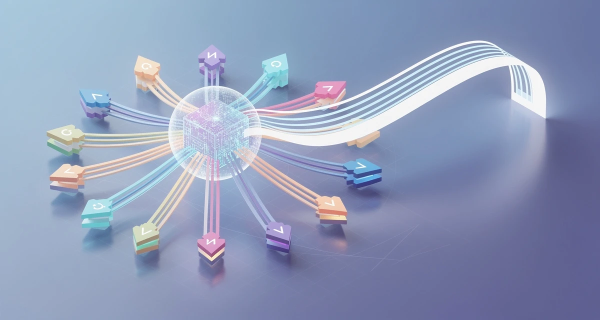
Multi-head attention is a transformer sublayer that runs h parallel attention operations, each with its own learned query, key, and value projections, then concatenates and linearly projects the results. This lets one transformer layer capture multiple distinct relationship types — syntax, semantics, coreference — simultaneously within the same parameter budget as a single head.
The motivation is straightforward: a single attention head can only learn one relevance pattern at a time. If one head learns subject-verb agreement, it cannot simultaneously specialize in coreference resolution. Multi-head attention solves this by running h heads in parallel, each with independent learned weight matrices, so the model develops a diverse set of attention patterns in one layer. The original transformer (Vaswani et al., 2017) used 8 heads; BERT Base uses 12; GPT-3 uses 96. Each head attends to a different aspect of the input, and the concatenated output gives the next layer a richer representation than any single head could produce.
This parallelism is what distinguishes multi-head attention from stacking attention layers. Two heads in one layer see the same input at the same depth, so they specialize without one head’s patterns being filtered through the other’s representation. For the architectural context of how these blocks fit together with positional encoding and layer normalization, see our transformer architecture breakdown.
Single-Head Attention: The Starting Point
To understand why multi-head attention matters, it helps to see the single-head case it generalizes. In single-head scaled dot-product attention, the input is projected once into query (Q), key (K), and value (V) matrices using learned weight matrices W_Q, W_K, and W_V. The attention output is computed as:
Attention(Q, K, V) = softmax(QK^T / √d_k) V
The result is a weighted blend of the value vectors, where the weights reflect how relevant each input position is to each query position. The softmax normalizes scores to a probability distribution, and the √d_k scaling keeps dot products stable as the key dimension grows. This single computation captures one set of relevance relationships across the full sequence. The scaling matters because without it, large dot products push softmax into saturation regions with vanishing gradients, which stalls learning.
From Single-Head to Multi-Head
Multi-head attention generalizes single-head attention by running the entire QKV computation h times in parallel, each with independent learned projections. Instead of one set of W_Q, W_K, W_V, the model learns h sets. Each head i computes:
head_i = Attention(Q W_Q^i, K W_K^i, V W_V^i)
The h head outputs are concatenated along the feature dimension and multiplied by a final output weight matrix W_O:
MultiHead(Q, K, V) = Concat(head_1, …, head_h) W_O
The key design choice is that the head dimension d_k is set to d_model / h. With model dimension 768 and 12 heads, each head operates on a 64-dimensional subspace. The total parameter count for the Q, K, V, and output projections is identical to a single head of dimension 768 — multi-head reparameterizes the same capacity into parallel subspaces rather than adding parameters. This is why increasing head count at fixed model dimension does not inflate the parameter budget, a property that matters for the cost discussion later.
How Multi-Head Attention Works Step by Step
The multi-head computation runs four steps per layer: project the input into h sets of Q, K, V matrices; compute scaled dot-product attention independently per head; concatenate the h outputs along the feature dimension; and apply a final learned output projection. All steps are differentiable and run in parallel on GPU hardware.
Step 1: Linear Projections into Q, K, V
Each head projects the shared input into its own Q, K, V matrices. For a model with dimension d_model and h heads, each head uses weight matrices W_Q^i, W_K^i, and W_V^i of shape (d_model, d_k), where d_k = d_model / h. The projections are standard linear transformations — matrix multiplies with learned weights. A BERT Base layer with d_model = 768 and 12 heads projects the input into 12 sets of 64-dimensional Q, K, V vectors. These projections are what let each head specialize: because each head learns different weights, it attends to different aspects of the input. The projection step is the source of the “multi” in multi-head attention.
Step 2: Scaled Dot-Product Attention per Head
Each head independently computes scaled dot-product attention. The query and key matrices are dot-producted, divided by √d_k, passed through softmax to produce attention weights, and multiplied by the value matrix. This produces a context-weighted output for each head. The computation is identical to single-head attention, just operating on a smaller-dimensional subspace. Because the heads are independent, they all run in parallel — a property that makes multi-head attention well-suited to GPU acceleration and a structural reason transformers train faster than the recurrent networks they replaced.
Step 3: Concatenation
The h head outputs, each of shape (sequence_length, d_k), are concatenated along the feature dimension into a single tensor of shape (sequence_length, d_model). This concatenation preserves all the distinct relationship patterns each head learned. A 12-head BERT layer produces 12 context vectors per position; concatenation assembles them into one 768-dimensional vector per position. This is the step where the parallel subspaces are recombined into the model’s working representation.
Step 4: Output Projection
The concatenated tensor is multiplied by a learned output weight matrix W_O of shape (d_model, d_model), producing the final multi-head attention output. This projection lets the model learn how to mix information across heads — which head outputs to emphasize, which to suppress, and how to combine them into a representation useful for the next layer. After this step, the output passes through a residual connection and layer normalization before reaching the feedforward sublayer of the transformer block.
Pro tip: When debugging a custom transformer implementation, the output projection W_O is the most common source of shape errors. Verify that the concatenated head dimension equals d_model before the projection — if head count does not evenly divide d_model, the concatenation step silently produces the wrong shape.
Computational Cost
The multi-head attention computation has the same asymptotic cost as single-head attention at fixed d_model: O(n² · d_model) for the attention scores, where n is the sequence length. Head count is a free architectural choice from a parameter-count perspective — the cost is in memory bandwidth during inference, not in the parameter budget. The practical cost driver is the key-value cache, which stores K and V tensors for all previously generated tokens so autoregressive generation does not recompute them. This cache grows with sequence length and head count and is the dominant cost in serving LLMs at scale — the motivation for the Multi-Query and Grouped-Query variants below.
How Many Heads Does a Model Need?
Head count is set so that head dimension (d_model divided by h) stays between 64 and 128. BERT Base uses 12 heads of dimension 64; GPT-3 uses 96 of dimension 128; LLaMA 2 uses 32 of dimension 128. Too many heads shrink each until it cannot express meaningful patterns; too few lose the parallel diversity that makes multi-head attention effective.
The Head Dimension Constraint
The per-head dimension d_k = d_model / h determines how expressive each head can be. If d_k is too small, each head operates in a subspace too narrow for meaningful attention patterns. If too large, fewer heads means less diversity. Empirically, most production transformers keep d_k between 64 and 128. BERT Base (768, 12 heads) uses d_k = 64. GPT-3 (12288, 96 heads) uses d_k = 128. LLaMA 2 7B (4096, 32 heads) uses d_k = 128. The pattern: designers choose a target d_k and set head count to match the model dimension. A model with d_model 512 and 64 heads would have d_k = 8 — a clear misconfiguration.
Head Count in Production Models
| Model | Model Dimension | Heads | Head Dimension | Total Attention Parameters |
|---|---|---|---|---|
| BERT Base | 768 | 12 | 64 | ~2.4M |
| BERT Large | 1024 | 16 | 64 | ~6.3M |
| GPT-3 175B | 12288 | 96 | 128 | ~680M |
| LLaMA 2 7B | 4096 | 32 | 128 | ~34M |
| LLaMA 2 70B | 8192 | 64 | 128 | ~201M |
| Mistral 7B | 4096 | 32 | 128 | ~34M |
The parameter column counts the Q, K, V, and output projections per layer. Notice that GPT-3’s 96 heads at d_k = 128 gives the same head dimension as LLaMA 2’s 32 heads — the larger model uses more heads to process a wider model dimension, not to increase per-head expressiveness. This is the general pattern: head count scales with model dimension, not independently of it.
Head Specialization: What Heads Actually Learn
One of the more studied properties of multi-head attention is that individual heads specialize during training without being explicitly directed to. Analyses of BERT (Clark et al., 2019) and GPT-2 (Voita et al., 2019) found that some heads consistently attend to specific syntactic relationships — subject-verb agreement, coreference resolution, positional patterns — while other heads turn out to be redundant or barely used. This emergent specialization is evidence that the multi-head design works: the parallel subspaces develop distinct functions during training.
“We observe that attention heads specialize: some heads focus on syntactic dependencies, others on rare words, and others on positional patterns — and that many heads can be pruned at inference time with minimal accuracy loss.” — Adapted from Voita et al., 2019
This specialization has a practical consequence: head pruning research shows that 30–50% of heads in a trained transformer can be removed with minimal impact on accuracy. The implication for inference cost is significant — if many heads are redundant, serving infrastructure can skip them, a finding that motivated the Multi-Query and Grouped-Query Attention variants below. For business teams, this means that a model advertising “96 attention heads” is not necessarily using all 96 productively; the effective number is often lower.
Choosing Head Count for a Custom Model
Most teams will use a pre-trained model rather than designing a transformer from scratch. But head count still matters when selecting open-weights models for self-hosting. The practical guidance:
- Keep per-head dimension between 64 and 128. Below 64, heads lose expressiveness; above 128, you trade away head diversity.
- Set head count to d_model / target_d_k. If d_model is 4096 and you want d_k of 128, use 32 heads.
- Do not add heads at the expense of model dimension. A wider model with fewer heads usually outperforms a narrow model with many heads.
Multi-Query and Grouped-Query Attention
Multi-Query Attention (MQA) shares one K and V projection across all heads, cutting the inference key-value cache by a factor of h. Grouped-Query Attention (GQA) shares K and V across groups of heads — the middle ground between full multi-head and MQA. Both reduce serving memory bandwidth, the dominant cost in LLM inference, with minimal quality loss.
The Key-Value Cache Problem
In autoregressive decoding, each new token attends to all previously generated tokens. To avoid recomputing the K and V projections for prior tokens at every step, the model stores them in a cache that grows linearly with sequence length. For a model with h heads, d_k head dimension, and L sequence length, the cache stores 2 × h × d_k × L values (K and V for each head, each token). For LLaMA 2 70B (64 heads, d_k 128, d_model 8192), a 4096-token sequence requires roughly 4GB of KV cache per request in fp16. At scale, this cache — not the compute — is the binding constraint on how many concurrent requests a serving system can handle. Memory bandwidth, the rate at which the GPU can move these cached tensors, becomes the inference bottleneck for long sequences and high batch sizes.
Multi-Query Attention (MQA)
Multi-Query Attention, introduced by Shazeer at Google in 2019 (arXiv:1911.02150), shares a single K and V projection across all heads. Each head still has its own Q projection, so queries remain head-specific, but all heads attend to the same keys and values. This reduces the KV cache by a factor of h: a 32-head model goes from 32 sets of K and V to 1. The inference speedup is substantial for long sequences, where KV cache memory bandwidth dominates. The trade-off is a modest quality drop — shared K and V projections reduce the diversity of what heads can attend to, and benchmark accuracy typically falls by 1–3% compared to standard multi-head attention. MQA is used in models like PaLM and some GPT variants where serving cost is prioritized over the last few percent of accuracy.
Grouped-Query Attention (GQA)
Grouped-Query Attention, introduced by Ainslie et al. at Google in 2023 (arXiv:2305.13245), is the middle ground. Instead of one shared K and V (MQA) or h independent K and V (standard MHA), GQA uses g groups, where each group of heads shares a K and V projection. With g = 1, GQA reduces to MQA; with g = h, GQA reduces to standard multi-head attention. The optimal is typically somewhere between: LLaMA 2 70B uses 8 groups for 64 heads, an 8x KV cache reduction with quality close to full MHA. GQA has become the default for new open-weights models because it recovers most of MQA’s inference savings while keeping the quality drop negligible.
MHA vs MQA vs GQA Comparison
| Variant | K/V Projections | KV Cache Size | Inference Speed | Quality vs MHA | Used By |
|---|---|---|---|---|---|
| Multi-Head Attention (MHA) | One per head | 2 × h × d_k × L | Baseline | Baseline | BERT, GPT-3, original Transformer |
| Multi-Query Attention (MQA) | One shared | 2 × d_k × L | Fastest | −1 to −3% | PaLM, some GPT variants |
| Grouped-Query Attention (GQA) | One per group (g groups) | 2 × g × d_k × L | Near MQA | −0 to −1% | LLaMA 2, Mistral, Gemma |
For business teams, the practical signal is in the “Used By” column. If you are self-hosting an open-weights model, GQA models (LLaMA 2, Mistral) will serve more concurrent requests on the same GPU than MHA models of the same parameter count. If you are buying API access, the savings are already baked into the provider’s per-token pricing. Either way, the attention variant is a meaningful cost variable, not a technical footnote.
What Multi-Head Attention Means for Business AI
Attention architecture determines inference cost, context window viability, and the number of concurrent requests a GPU can handle. Head count, head dimension, and the attention variant (MHA, MQA, or GQA) are spec-sheet variables business teams can read directly when choosing between open-weights models or evaluating LLM API providers.
Model Selection: Head Count as a Quality Signal
When comparing open-weights models for self-hosting, head count and attention variant are part of the spec sheet, and they affect both quality and cost. A model with a reasonable head dimension (64–128) and GQA will generally offer a better cost-quality ratio than one with tiny heads or full MHA at the same parameter count. According to McKinsey Global Institute (2023, “The Economic Potential of Generative AI”), generative AI could add $2.6 trillion to $4.4 trillion annually across use cases, with customer operations and marketing as the highest-value applications — and every dollar of that estimate runs through attention computation. The models that deliver that value most cost-effectively are the ones whose attention architecture is tuned for the deployment scenario, not just the benchmark.
Inference Cost and the KV Cache
For teams self-hosting models, the KV cache is the inference cost variable most affected by the attention variant. A 7B-parameter MHA model with 32 heads and a 4096-token context requires roughly 1GB of KV cache per request in fp16. The same model with GQA (8 groups) needs roughly 256MB — a 4x reduction that directly increases the number of concurrent requests a single GPU can handle. This is why GQA has become the default in new open-weights releases: it does not change the model’s benchmark quality meaningfully, but it changes the serving economics substantially. For a business running hundreds of concurrent inference requests, the attention variant can be the difference between needing 4 GPUs and needing 16.
Context Window and Attention Efficiency
Context window size — the maximum tokens a model can process in one request — is constrained by attention’s quadratic memory scaling and KV cache size. Flash Attention (Dao et al., 2022) addressed the training-side memory problem by tiling attention computation to fit in GPU SRAM, achieving 10–20x memory reduction with identical results. On the inference side, GQA and MQA address the KV cache. Together, these advances are why production context windows now range from 32K (Claude 3 Haiku) to 200K (Claude 3.5 Sonnet) to 2M (Gemini 1.5 Pro), as documented in the Stanford HAI AI Index 2024. Match context window to actual document lengths: 8K handles most chatbot turns, 32K–100K handles report analysis, and 128K+ is for full contract or codebase review.
What to Ask a Vendor
When evaluating an LLM API or self-hostable model, the attention architecture is a legitimate line of questioning:
- Does the model use MHA, MQA, or GQA? This tells you whether per-token pricing reflects inference efficiency gains or an older, less efficient architecture.
- What is the head dimension? Below 64 suggests the model trades per-head expressiveness for marketing-friendly head counts.
- How does the KV cache scale with context length? This determines how cost scales when you send long documents.
- Is Flash Attention used in the training and serving stack? Its absence signals older infrastructure.
Ready to evaluate AI models for your business? GrowthGear’s team has helped 50+ startups select and deploy transformer-based AI systems, from document analysis to customer service automation. Book a Free Strategy Session to map the right model architecture to your actual use case and budget.
Cross-Domain Attention: Beyond Language
Multi-head attention is not language-specific. The same architecture powers vision transformers (ViT), where image patches take the role of tokens; audio models like Whisper; and protein-structure models like AlphaFold 2. For business applications in visual search, document understanding, or multimodal support, the same head-count and attention-variant trade-offs apply. Teams applying attention-based models to digital marketing automation or sales conversion workflows benefit from understanding that the underlying component is the same across modalities.
Summary: Multi-Head Attention at a Glance
| Concept | What It Does | Why It Matters for Business |
|---|---|---|
| Multi-Head Attention | Runs h parallel attention heads with independent projections | Captures multiple relationship types in one layer; core of every transformer |
| Head Dimension (d_k) | Per-head subspace size = d_model / h | Below 64 loses expressiveness; 64–128 is the production range |
| Head Count (h) | Number of parallel attention operations | Scales with model dimension, not independently; more heads ≠ more capacity at fixed d_model |
| Scaled Dot-Product | softmax(QK^T / √d_k) V per head | The core attention computation; scaling keeps gradients stable |
| Output Projection (W_O) | Mixes concatenated head outputs | Lets the model learn how to combine head contributions |
| Multi-Query Attention (MQA) | Shares one K and V across all heads | Cuts KV cache by h; used when serving cost dominates |
| Grouped-Query Attention (GQA) | Shares K and V across g groups | Default for new open-weights models; near-MHA quality at near-MQA cost |
| KV Cache | Stores K and V for prior tokens during decoding | Dominant inference memory cost; scales with sequence length and head count |
For teams building on top of transformers rather than designing them, the takeaway is that attention architecture is a cost and quality variable you can read off a model’s spec sheet. For a deeper grounding in the full transformer stack, see our guides on transformer architecture and BERT in NLP.
Take the Next Step
Multi-head attention is not a detail you can afford to skip when evaluating AI vendors or choosing between open-weights models. The head count, head dimension, and attention variant (MHA, MQA, or GQA) directly determine inference cost, context window viability, and the number of concurrent requests your infrastructure can handle. Whether you are selecting an LLM API, planning to self-host, or building document-processing automation, understanding this component lets you ask the questions that separate an efficient deployment from an expensive one.
GrowthGear has helped 50+ startups cut through vendor specifications and deploy transformer-based AI systems that fit their actual workloads and budgets. If you are ready to match the right attention architecture to your real inference needs, let’s talk.
Book a Free Strategy Session →
Sources & References
- Vaswani et al., Google Brain — “Attention Is All You Need” — Introduced multi-head attention and the full transformer architecture; 8-head model achieved 28.4 BLEU on WMT 2014 EN-DE translation (2017)
- Shazeer, Google — “Fast Transformer Decoding: One Write-Head is Enough” — Introduced Multi-Query Attention, sharing one K and V projection across all heads to reduce KV cache memory bandwidth during inference (2019)
- Ainslie et al., Google — “GQA: Training Generalized Multi-Query Transformer Models for Multi-Attention” — Introduced Grouped-Query Attention as the middle ground between MHA and MQA; adopted by LLaMA 2, Mistral, and Gemma (2023)
- Stanford HAI AI Index Report 2024 — Documented context window growth from 4,096 tokens (GPT-3, 2020) to 2M+ tokens (Gemini 1.5 Pro, 2024), driven by attention efficiency improvements
- McKinsey Global Institute — “The Economic Potential of Generative AI” (2023) — Estimated generative AI could add $2.6–4.4 trillion annually; customer operations and marketing identified as highest-value applications
Frequently Asked Questions
Multi-head attention is a transformer component that runs several scaled dot-product attention operations in parallel, each with its own learned query, key, and value projections. The head outputs are concatenated and linearly projected, letting the model capture different relationship types — syntax, semantics, coreference — in a single layer.
Each head projects the input into separate Q, K, V matrices using learned weights, computes scaled dot-product attention independently, and produces a context vector. All head outputs are concatenated along the feature dimension and multiplied by a final output weight matrix W_O to produce the layer result.
BERT Base uses 12 heads, GPT-3 uses 96, and LLaMA 2 uses 32. Head count trades representational diversity against per-head dimension: too few heads underfit relationships, too many shrink each head's dimension until it cannot express meaningful patterns. Most production models keep head dimension between 64 and 128.
Multi-head attention gives each head its own Q, K, and V projections. Multi-Query Attention (MQA) shares one K and V projection across all heads, cutting memory bandwidth during inference by roughly the head count. Grouped-Query Attention (GQA) is the middle ground, sharing K and V across groups of heads.
Scaling by the square root of the key dimension keeps dot-product magnitudes stable as dimension grows. Without scaling, dot products into large key dimensions push softmax into regions with tiny gradients, which stalls training. The scale factor makes attention learnable across the wide dimension ranges transformers use.
No, not when head count and head dimension multiply to the model dimension. A model with dimension 768 and 12 heads of dimension 64 uses the same total projection parameter count as one head of dimension 768. Multi-head reparameterizes the same capacity into parallel subspaces rather than adding capacity.
No. Multi-head attention is used in vision transformers (ViT), audio models like Whisper, protein-structure models like AlphaFold 2, and diffusion model U-Nets. Any transformer-based architecture, regardless of modality, relies on multi-head attention to capture multi-scale relationships in parallel.